Quarto enables you to weave together content and executable code into a finished document. To learn more about Quarto see https://quarto.org.
Background of the example
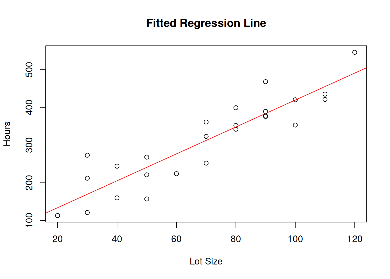
The Toluca Company manufactures refrigeration equipment as well as many replacement parts. In the past, one of the replacement parts has been produced periodically in lots of varying sizes.
When a cost improvement program was undertaken, company officials wished to determine the optimum lot size for producing this part.
The production of this part involves setting up the production process (which must be done no matter what is the lot size) and machining and assembly operations.
One key input for the model to ascertain the optimum lot size was the relationship between lot size and the labor hours required to produce the lot.
To determine this relationship, data on lot size and work hours for 25 recent production runs were utilized.
The production conditions were stable during the six-month period in which the 25 runs were made and were expected to continue to be the same during the next three years, the planning period for which the cost inprovement program was being conducted.
# Scan a data set into R # Change the working directory to the appropriate one # Also before scan the data set into R, check the data set first to see # the number of columns it has, you need it for assigning ncol below.ch01ta01<-matrix(scan("CH01TA01.txt"),ncol=2, byrow=T);ch01ta01
# Load Mass package to construct confidence intervals for# beta'sconfint(fm) # conf. int.'s for reg. coeff.'s default: 95% #
               2.5 %     97.5 %
(Intercept) 8.213711 116.518006
x           2.852435   4.287969
confint(fm, level=0.9)
                  5 %       95 %
(Intercept) 17.501100 107.230617
x            2.975536   4.164868
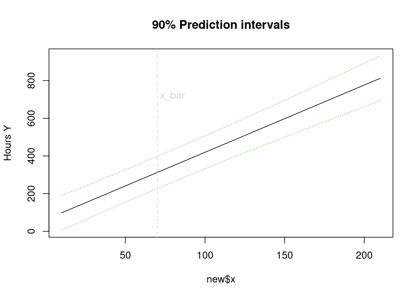
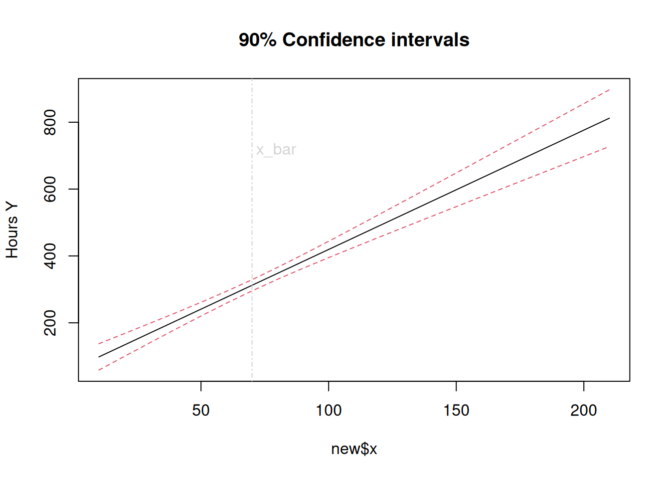
# Estimation of mean response, its confidence intervals Ex. on p. 55, p. 59# and prediction intervals # This is how you # construct confidence/prediction intervals for the mean response at given predictor x's valuesnew<-data.frame(x=seq(10,210,10))new
pred.w.plim <-predict(lm(y~x), new, interval="prediction",level=0.9)pred.w.clim <-predict(lm(y~x), new, interval="confidence",level=0.9)cbind(new$x,pred.w.plim) # prediction intervals for x at seq(10,210,10)
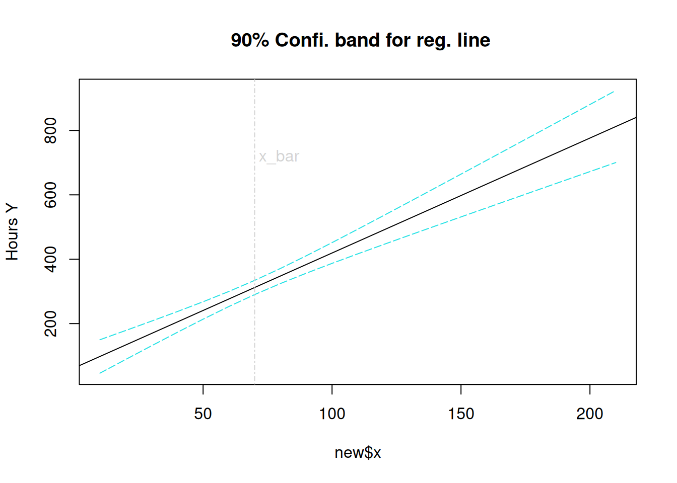
# Confidence band for the entire reg. line Ex. on p. 62, Fig. 2.6width<-function(n,xh,alpha){sqrt(2*qf(1-alpha,2,n-2)*sum((y-fitted(fm))^2)/(n-2)*(1/n+(xh-mean(x))^2/((n-1)*var(x))))}n<-length(y)u<-coef(fm)[1]+coef(fm)[2]*new$x+width(n,new$x,0.1)l<-coef(fm)[1]+coef(fm)[2]*new$x-width(n,new$x,0.1)band<-cbind(l,u)cbind(new$x,band)
# Graphical displaymatplot(new$x,band,col=c(5,5),lty=c(5,5),type="l", #ylim=c(70,500),main=" 90% Confi. band for reg. line",ylab="Hours Y")abline(coef(fm),col=1)abline(v=mean(x), col="lightgray", lty=4);text(70,700, "x_bar",col="lightgray",adj=c(-.1,-.1))
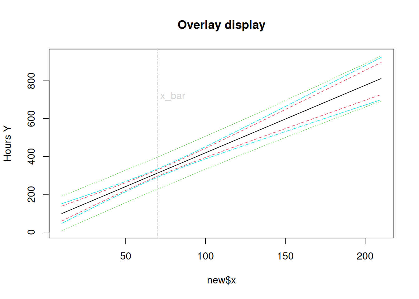
# It is hard to compare among plots......# Graphical display these intervals for easy comparison # Overlay CI, PI, Conf band at those x valuesmatplot(new$x,cbind(pred.w.clim, pred.w.plim[,-1],band),col=c(1,2,2,3,3,5,5), lty=c(1,2,2,3,3,5,5),type="l", main="Overlay display",ylab="Hours Y")abline(v=mean(x), col="lightgray", lty=4);text(70,700, "x_bar",col="lightgray",adj=c(-.1,-.1))
# Before you quit R, clean up the objects, please. #detach()# rm(list=ls())# q()# Also try the "Save History" under "File" of the R Console window,# and you may find out how Yes prepare these handouts..... :> #