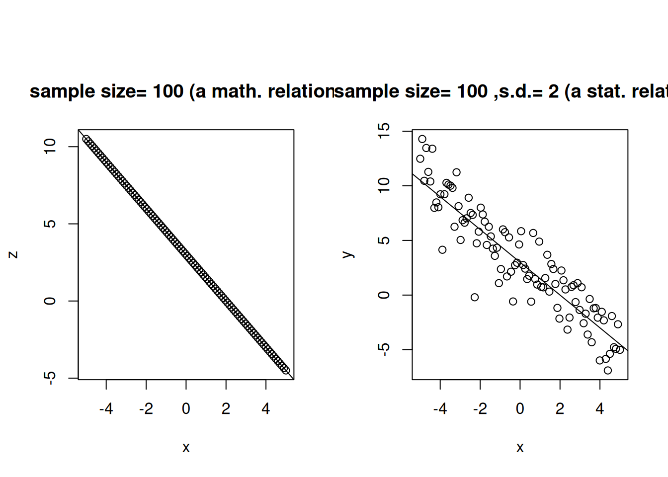
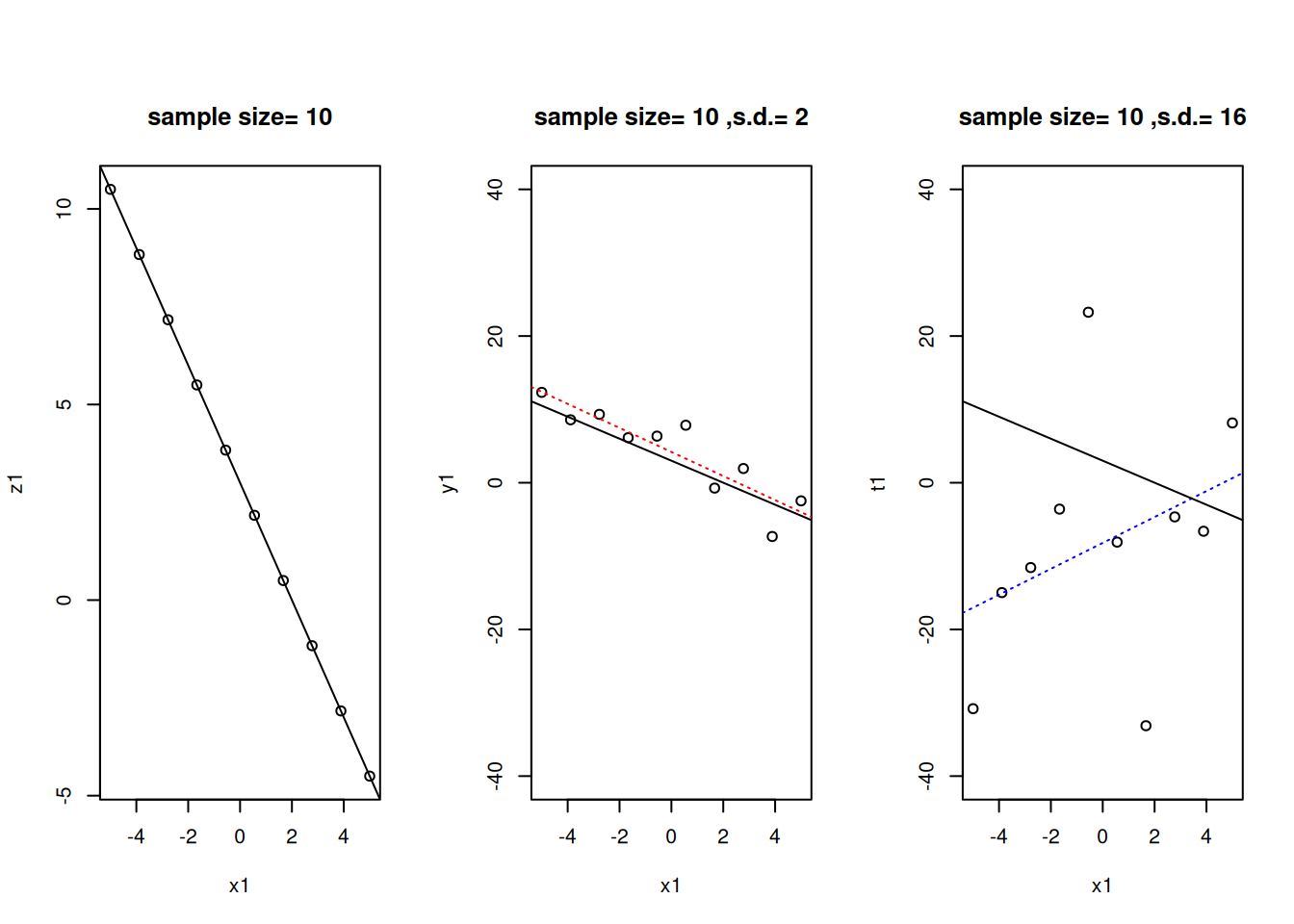
z <- a+b*x; # a: intercept, b: slope #plot(x,z,main=paste("sample size=", n1, "(a math. relation)"));abline(a, b, lty=1,col=1); # The true regression line #sd1 <-2y<-z+rnorm(n1)*sd1; # rnorm(M) gives you M random numbers from N(0,1) #plot(x,y, main=paste("sample size=",n1, ",s.d.=", sd1, "(a stat. relation)" ));abline(a, b, lty=1,col=1); # The true regression line #
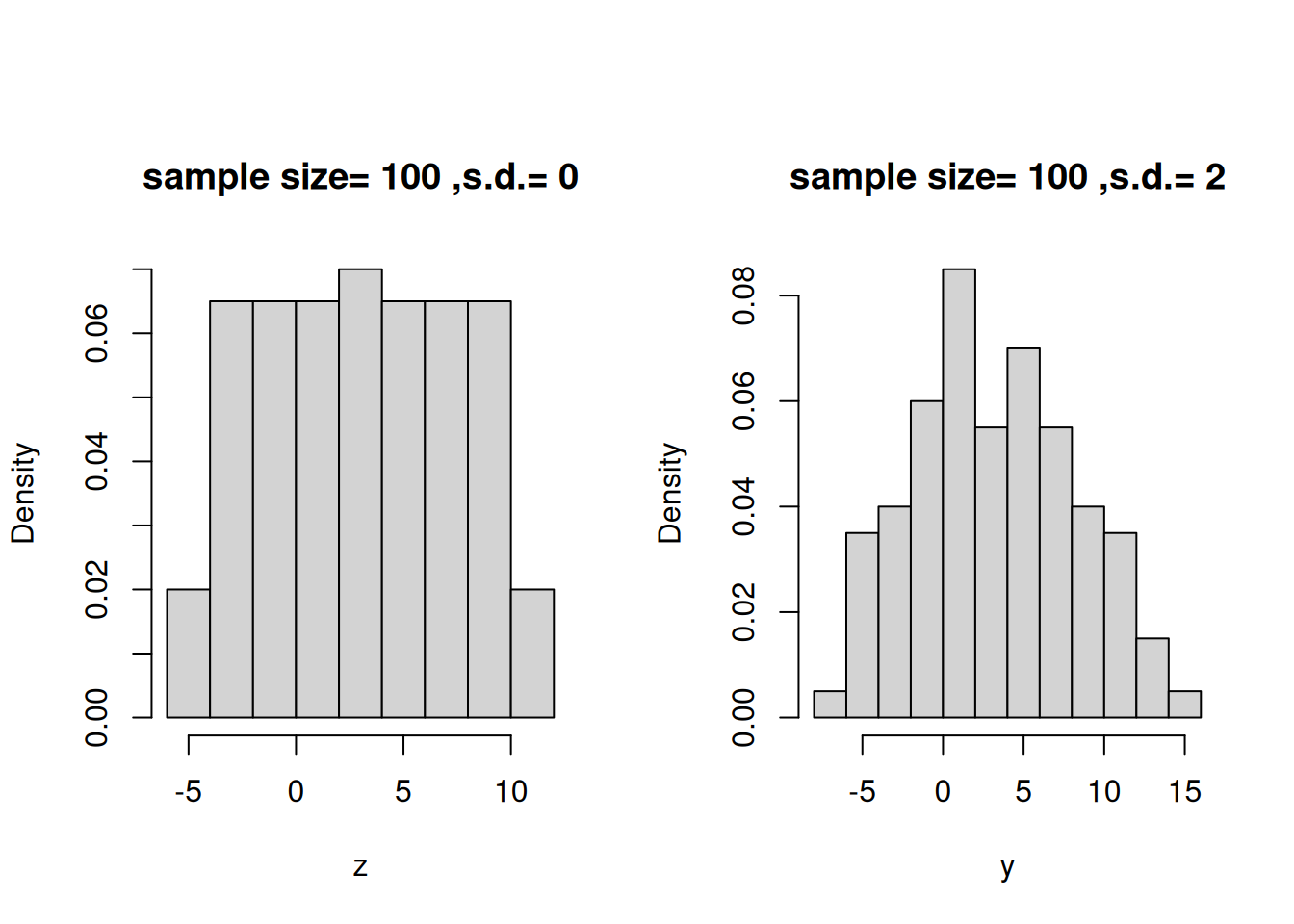
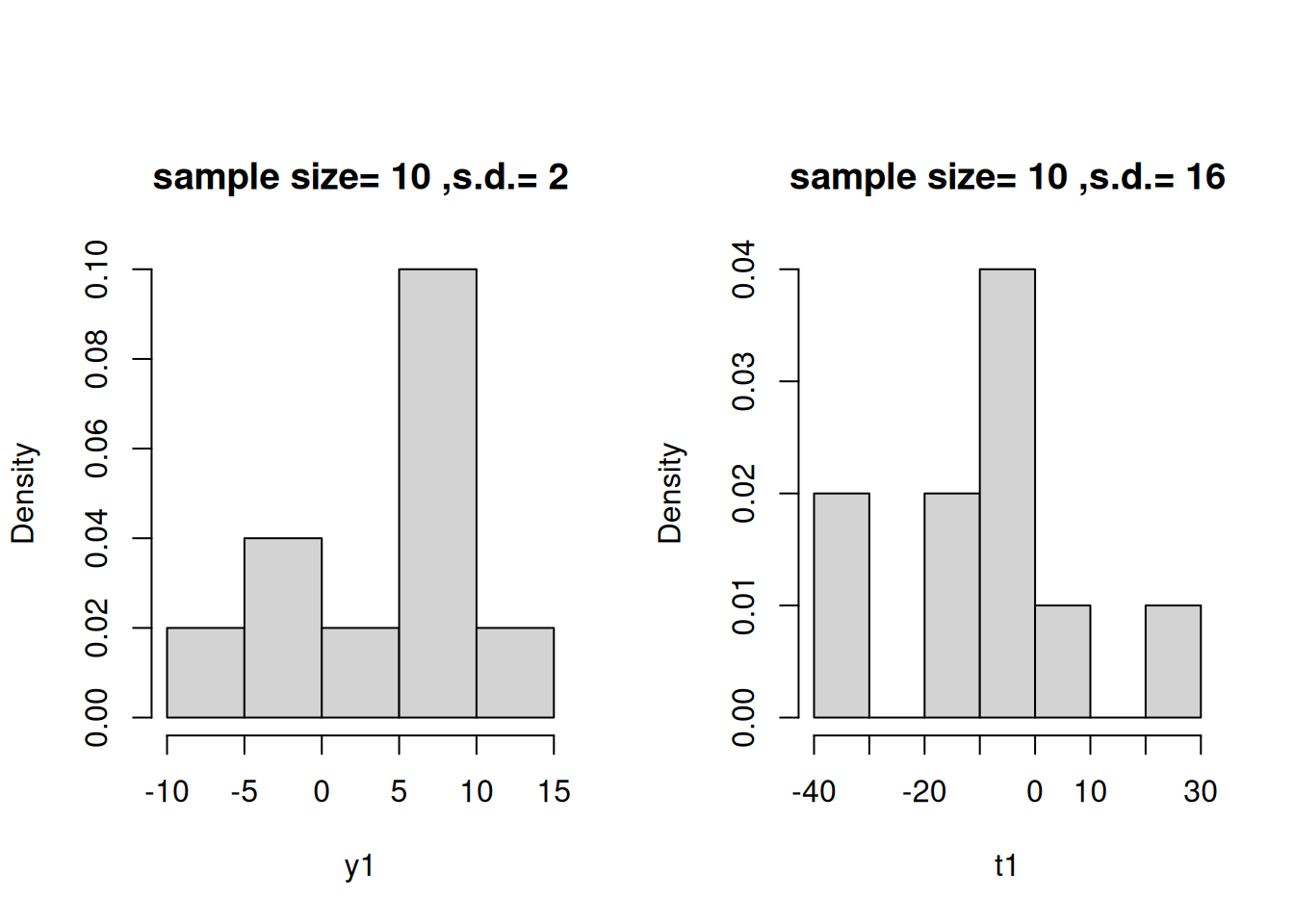
opar <-par(mfrow =c(1,2), oma =c(0, 0, 2.7, 0)); hist(z,freq=FALSE, main=paste("sample size=",n1, ",s.d.=", 0)) # Histogram of z's #hist(y,freq=FALSE, main=paste("sample size=",n1, ",s.d.=", sd1)) # Do you see any difference in these two histograms? #
You can add options to executable code like this
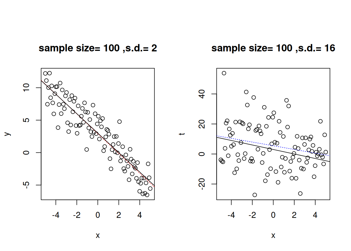
opar <-par(mfrow =c(1,2), oma =c(0, 0, 2.7, 0)); y<-z+rnorm(n1)*sd1;plot(x,y, main=paste("sample size=",n1, ",s.d.=", sd1));fm <-lm(y~x); # Simple regression; y regress on x # summary(fm); # Check if estimates for intercept and slope good #
Call:
lm(formula = y ~ x)

Residuals:
    Min      1Q  Median      3Q     Max
-4.8466 -1.3047 -0.0912  1.5445  5.0028

Coefficients:
            Estimate Std. Error t value Pr(>|t|)
(Intercept)  2.92370    0.19170   15.25   <2e-16 ***
x           -1.52351    0.06575  -23.17   <2e-16 ***
---
Signif. codes:  0 '***' 0.001 '**' 0.01 '*' 0.05 '.' 0.1 ' ' 1

Residual standard error: 1.917 on 98 degrees of freedom
Multiple R-squared:  0.8457,    Adjusted R-squared:  0.8441
F-statistic:   537 on 1 and 98 DF,  p-value: < 2.2e-16
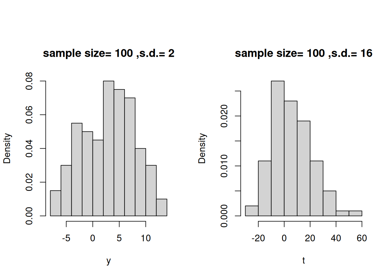
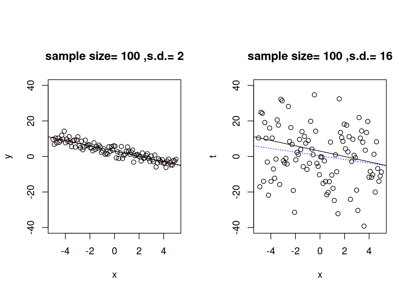
abline(fm, lty=3,col="red"); # Add the estimated reg. line to the current plot #abline(a, b, lty=1,col=1); # The true regression line #sd2 <-16;t<-z+rnorm(n1)*sd2;plot(x,t,main=paste("sample size=",n1, ",s.d.=", sd2));abline(a, b, lty=1, col=1);fm1 <-lm(t~x);summary(fm1);
Call:
lm(formula = t ~ x)

Residuals:
    Min      1Q  Median      3Q     Max
-34.930 -11.756   0.275   9.198  42.584

Coefficients:
            Estimate Std. Error t value Pr(>|t|)
(Intercept)   5.4956     1.4586   3.768 0.000281 ***
x            -1.2288     0.5002  -2.457 0.015788 *
---
Signif. codes:  0 '***' 0.001 '**' 0.01 '*' 0.05 '.' 0.1 ' ' 1

Residual standard error: 14.59 on 98 degrees of freedom
Multiple R-squared:  0.058, Adjusted R-squared:  0.04839
F-statistic: 6.034 on 1 and 98 DF,  p-value: 0.01579
opar <-par(mfrow =c(1,2), oma =c(0, 0, 2.7, 0)); y<-z+rnorm(n1)*sd1;plot(x,y, main=paste("sample size=",n1, ",s.d.=", sd1),ylim=c(-40,40));fm <-lm(y~x); # Simple regression; y regress on x # summary(fm); # Check if estimates for intercept and slope good #
Call:
lm(formula = y ~ x)

Residuals:
    Min      1Q  Median      3Q     Max
-4.0602 -1.2436 -0.1034  1.4741  5.3235

Coefficients:
            Estimate Std. Error t value Pr(>|t|)
(Intercept)  3.01993    0.19426   15.55   <2e-16 ***
x           -1.43900    0.06662  -21.60   <2e-16 ***
---
Signif. codes:  0 '***' 0.001 '**' 0.01 '*' 0.05 '.' 0.1 ' ' 1

Residual standard error: 1.943 on 98 degrees of freedom
Multiple R-squared:  0.8264,    Adjusted R-squared:  0.8246
F-statistic: 466.5 on 1 and 98 DF,  p-value: < 2.2e-16
abline(fm, lty=3,col="red"); # Add the estimated reg. line to the current plot #abline(a, b, lty=1,col=1); # The true regression line #anova(fm); # Obtain the ANOVA table #
Analysis of Variance Table

Response: y
          Df  Sum Sq Mean Sq F value    Pr(>F)
x          1 1760.46 1760.46  466.51 < 2.2e-16 ***
Residuals 98  369.82    3.77
---
Signif. codes:  0 '***' 0.001 '**' 0.01 '*' 0.05 '.' 0.1 ' ' 1
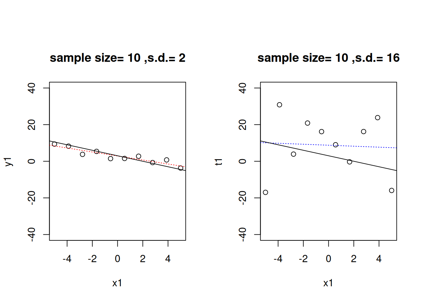
Call:
lm(formula = t1 ~ x1)

Residuals:
    Min      1Q  Median      3Q     Max
-27.072  -7.881   3.840  10.788  21.049

Coefficients:
            Estimate Std. Error t value Pr(>|t|)
(Intercept)   8.7635     5.4121   1.619    0.144
x1           -0.2665     1.6958  -0.157    0.879

Residual standard error: 17.11 on 8 degrees of freedom
Multiple R-squared:  0.003077,  Adjusted R-squared:  -0.1215
F-statistic: 0.02469 on 1 and 8 DF,  p-value: 0.879
anova(fm3); #the ANOVA table #
Analysis of Variance Table

Response: t1
          Df  Sum Sq Mean Sq F value Pr(>F)
x1         1    7.23   7.232  0.0247  0.879
Residuals  8 2343.30 292.912
# Can you see the effect of sample size and standard deviation on the fitted line? ## Play with R as much as possible this week, you will need to use R # for your homework shortly. # Always remove all objects before ending your R session # # rm(list=ls(all=TRUE));# q() # To quit R ## Come to my office if you have any question! ^_^ Yes.