Rgames: Week 7-2 (revised)

Here we will use Stat 2016 midterm data to further illustrate the related modelling and analysis of a exam score data set.
Curator/Coder: Kno Tsao

Import raw data

Now we load the raw data (names/id removed and reordered for privacy and anonymity) from the web and reconstruct the summary statistics and graphs given in 2016 Stat Website(plots)

Local data import and analyses

If you have got the data set stat2016.txt on your local folder, you can change the working directory to the folder where data is and then proceed

t<-matrix(scan("stat2016.txt"),ncol=3,byrow=T)

Read 189 items

summary(t) # This is not the way to summarize data, just for comparison. 

       V1              V2               V3        
 Min.   :2.000   Min.   :  0.00   Min.   :-10.00  
 1st Qu.:2.000   1st Qu.: 25.50   1st Qu.: 13.50  
 Median :2.000   Median : 46.00   Median : 31.00  
 Mean   :2.476   Mean   : 46.52   Mean   : 34.11  
 3rd Qu.:3.000   3rd Qu.: 67.50   3rd Qu.: 53.00  
 Max.   :5.000   Max.   :110.00   Max.   :100.00  

exam <-data.frame(year=as.factor(t[,1]),mid=t[,2],final=t[,3])
summary(exam)

 year        mid             final       
 2:42   Min.   :  0.00   Min.   :-10.00  
 3:15   1st Qu.: 25.50   1st Qu.: 13.50  
 4: 3   Median : 46.00   Median : 31.00  
 5: 3   Mean   : 46.52   Mean   : 34.11  
        3rd Qu.: 67.50   3rd Qu.: 53.00  
        Max.   :110.00   Max.   :100.00  

plot(exam)

Further plots on midterm and final scores

attach(exam)
stem(mid)

  The decimal point is 1 digit(s) to the right of the |

   0 | 011556056789
   2 | 01256770146779
   4 | 00046667901555558
   6 | 555500011555
   8 | 0501155
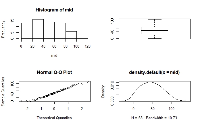
  10 | 0

par(mfrow=c(2,2));    # Setup the graphical device
hist(mid); boxplot(mid); qqnorm(mid);
plot(density(mid));

I use “mid” as the variable, you can try the command on “final”

stem(final)

  The decimal point is 1 digit(s) to the right of the |

  -0 | 00
   0 | 01344560111123456678
   2 | 013468001136677889
   4 | 01379133367788
   6 | 0335689
   8 | 3
  10 | 0

par(mfrow=c(2,2));    # Setup the graphical device
hist(final); boxplot(final); qqnorm(final);
plot(density(final));

Relation between mid and final

plot(final,mid,main="Final vs. Midterm Stat 2016")
m1<-lm(final~mid)
summary(m1)

Call:
lm(formula = final ~ mid)

Residuals:
    Min      1Q  Median      3Q     Max 
-36.062 -12.562  -3.029  10.211  61.213 

Coefficients:
            Estimate Std. Error t value Pr(>|t|)    
(Intercept)  8.44481    5.14339   1.642    0.106    
mid          0.55168    0.09554   5.774 2.79e-07 ***
---
Signif. codes:  0 ‘***’ 0.001 ‘**’ 0.01 ‘*’ 0.05 ‘.’ 0.1 ‘ ’ 1

Residual standard error: 20.54 on 61 degrees of freedom
Multiple R-squared:  0.3534,    Adjusted R-squared:  0.3428 
F-statistic: 33.34 on 1 and 61 DF,  p-value: 2.791e-07

# plot(m1)
abline(m1)

m1$coef

(Intercept)         mid 
   8.444807    0.551681 

Questions/Tasks

• Q1. Is final normal? Is final score appear normal? Your rationale? How do you make it “more normal”?
• Q2. Estimate the passing threshold. Focus on the final, suppose the instructor failed 1/3 of the class based solely on the final scores. If you want to estimate the passing threshold, should you transform or not? How do you do it exactly? What’s the difference between two approaches?
• Q3. If the course grade is based on cpoint = 0.35 mid + 0.65 final and the failing rate is about 1/3,
  • Estimate the passing threshold/point of cpoint
  • You and your roommates score 10, 30, 50, 70 in midterm respectively, what are the (estimated) final they need to score in order to pass?
• Mid-Project (Checkpoint: 5/1, A team =3~5 persons or ask Kno)
  • Given the 2016 Stat data set, estimate the final exam scores of 4 students who scores, say, 10, 30, 50, 70 (or more realistic scores of your interest) in the midterm Stat 2017.
  • According to an unidentified yet reliable source, the course grades given by instructor is roughly #A:#B:#C:#(D or E) \(\approx 1:3:3:3\). Estimate the course grades of these 4 students. Please provide the assumptions and rationale of your estimation.